
Machine Learning: An Introduction to CART Decision Trees in Ruby


In the middle of last year, we released an internal tool to help address a pretty significant issue. That is how the Pecas tool was born, and you can read about the Business Case for Pecas here .
Pecas relies on a binary classification machine learning model to classify time entries as valid or invalid. It is a combination of a Django app, that hosts the Slackbot and other data processing tasks, and a FastAPI app that hosts the machine learning model built using the Scikit-learn Python library. Scikit-learn provides a great set of classification models you can use, which are optimized and very robust, making it a solid choice to build your model. However, understanding the principles behind the classification can be a bit tricky, and machine learning models can feel a bit like a black box.
In this series, we’ll explore some principles of machine learning, namely binary classifiers, and walk through how they connect to each other, in Ruby. This article will focus on decision trees, namely CART (Classification And Regression Trees) and a little bit of the mathematics behind them.
A Brief Introduction to Decision Trees and Binary Classification
Decision trees are a very popular machine learning algorithm that belongs to the supervised learning category. They are quite flexible and can be used for both regression and classification tasks. We’ll focus on classification.
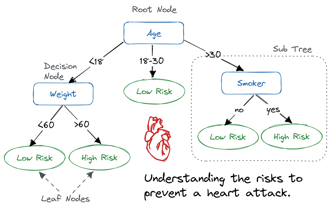
Example of a decision tree. Source: Decision Tree Classification in Python by DataCamp
Tree-based methods work by taking in a dataset and repeatedly dividing it into smaller groups. The main goal is to always divide the data in a way that makes the smaller groups as homogeneous as possible, that is, choose the split that results in the grouping with the most items from a single class. Before we dive into how decision trees work, let’s cover some concepts that will be used throughout this article:
Supervised learning: Refers to the group of Machine Learning techniques that predict an outcome based on labeled data. That is data that includes all the variables used for predictions (predictors) as well as the actual prediction (label) associated with each individual record.
Homogeneous data: Refers to a subset of data that belongs to a single class.
Class or Label: Each of the potential outcomes (or categories) in a classification task.
Regression: Type of supervised learning that involves predicting a continuous output variable based on one or more input features.
Classification: Type of supervised learning that involves predicting discrete labels (or categories) for a given input.
Binary classification: Refers to classification problems with two target classes.
Overfitting: When a Machine Learning model learns too much about the training data and loses its ability to generalise, performing poorly on unseen data.
Some important terms to keep in mind when working with decision trees are:
Root Node: Topmost node in the tree, representing the entire dataset. All branches originate from the root node.
Decision Node: Nodes within the tree where data is split. Can lead to another decision node or to a leaf node.
Leaf Node or Terminal Node: The final output of the decision process. Does not split further and contains the predicted label.
Pruning: Process of removing sub-nodes of a decision node, reducing the complexity of the tree. Used to reduce overfitting.
Depth of the Tree: The length of the longest path from the root node to a leaf node.
Impurity: A measure of how homogeneous the data is. Data is pure if it only contains a single class. The more classes in the data, the more impure it is. It varies between 0 and 1.
Information Gain: Measure how well a characteristic separates data into similar groups. Based on the decrease in impurity after a dataset is split on a particular attribute.
In binary classification, the recursive algorithm starts by choosing a feature based on which to split the data, and split it into two nodes. Then one or both of these nodes are split based on a different feature. And the process continues until a specific condition is met that stops the recursion.
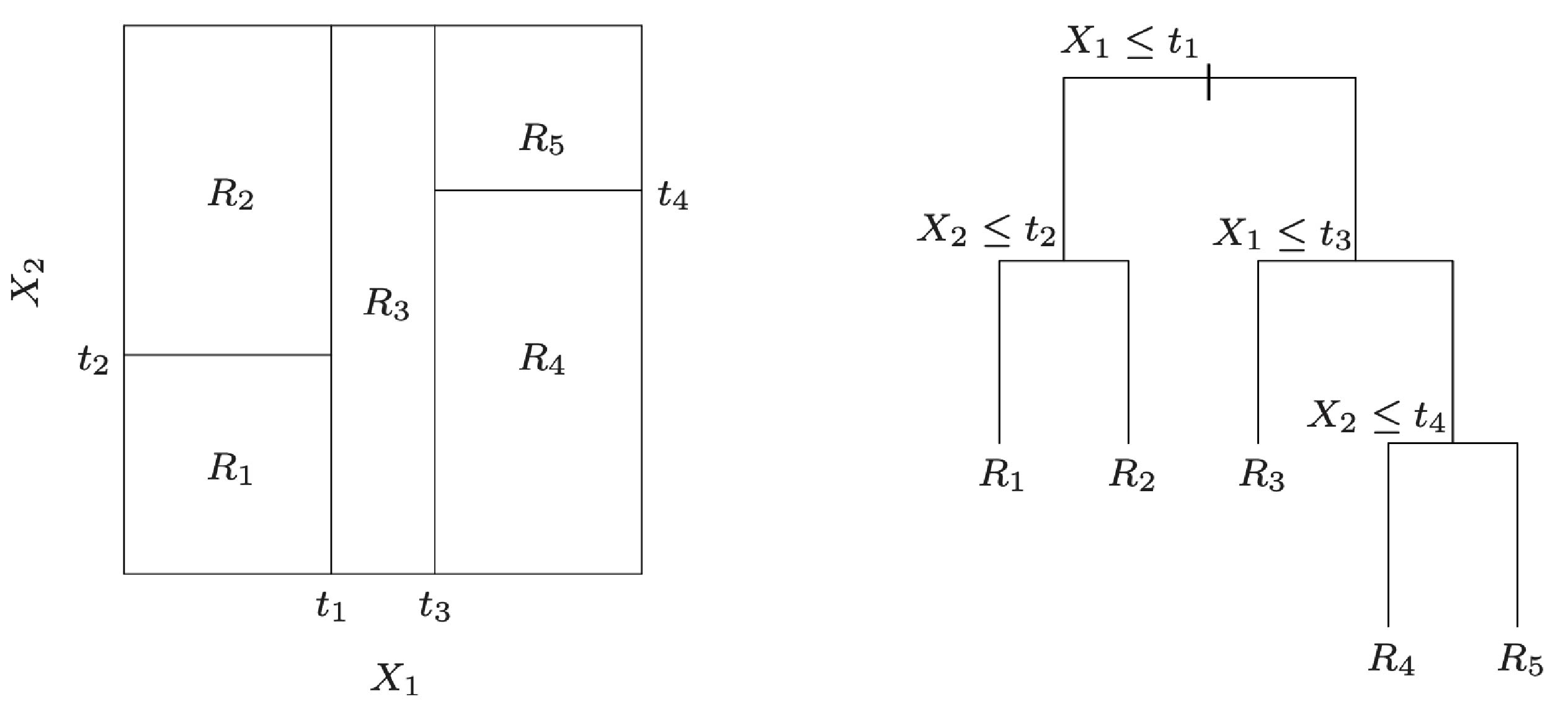
Partition of a two-dimensional feature space by recursive binary splitting and tree corresponding to the partition. Source: The Elements of Statistical Learning: Data Mining, Inference, and Prediction by Trevor Hastie, Robert Tibshirani and Jerome Friedman .
At each decision point, a feature and threshold are chosen. The threshold is the value of the feature where the split happens, that is, the value that actually splits the dataset.
Let’s imagine that we have a dataset of email data we’ll use to classify emails into spam or not spam. One of the features in the dataset, \(X_1\), is an integer indicating how many characters the email’s body has, and the best split happens at 900 characters. This means that \(t_1\) is 900, and emails with 900 or less characters will go into the left child node while emails with more than 900 characters will go into the right child node. In this case, email length in the feature chosen at the decision point, and 900 is the threshold.
The trained decision tree is then able to classify new inputs by traversing the tree from the root to a leaf node following the decisions at each internal node.
CART decision trees
There are different tree-based methods available, with the two most popular ones being CART (Classification and Regression Tree) and ID3 (Iterative Dichotomizer 3) with it’s evolution, C4.5. In this article, we’ll focus on the CART algorithm, considering we used a Scikit-learn classifier to build our model, and Scikit-learn uses an optimized version of the CART algorithm according to its documentation .
For detailed information about how CART and ID3 compare to each other, check out the Comparative Study ID3, CART and C4.5 Decision Tree Algorithm: A Survey by Sonia Singh and Priyanka Gupta .
CART decision trees are used for binary classification and can generate both classification and regression trees. They use the Gini Index as a measure of impurity, and the objective is to minimise the Gini index at each node.
The Gini Index is calculated as:
\[Gini(E) = 1 - \sum_{j=1}^Q p_j ^2\]It measures the probability that two randomly chosen individuals belong to different groups. The higher the Gini index, the more impurity in the data. For each node, a CART decision tree will calculate the Gini Index for different features, and choose the feature with the smallest value to split on, since the goal is to minimise impurity.
CART Decision Tree in Theory
Let’s look at a famous example that is used to explain decision trees, and see how CART applies it. Take this example dataset of weather data to determine whether there was gameplay or not:
| Outlook | Temperature | Humidity | Wind | Gameplay? |
|---|---|---|---|---|
| Sunny | High | High | Weak | False |
| Sunny | High | High | Strong | False |
| Cloudy | High | High | Weak | True |
| Rainy | Mild | High | Weak | True |
| Rainy | Low | Normal | Weak | True |
| Rainy | Low | Normal | Strong | False |
| Cloudy | Low | Normal | Strong | True |
| Sunny | Mild | High | Weak | False |
| Sunny | Low | Normal | Weak | True |
| Rainy | Mild | Normal | Weak | True |
| Sunny | Mild | Normal | Strong | True |
| Cloudy | Mild | High | Strong | True |
| Cloudy | High | Normal | Weak | True |
| Rainy | Mild | High | Strong | False |
To start building the tree, we need to identify how to split the root node. To do that, we calculate the Gini Index for
each feature and pick the one with the smallest index. Let’s take, for example, the Outlook feature:
| Outlook | Gameplay | No Gameplay | Total Instances |
|---|---|---|---|
| Sunny | 2 | 3 | 5 |
| Cloudy | 4 | 0 | 4 |
| Rainy | 3 | 2 | 5 |
To calculate the Gini Index, we calculate the index for each possible value and then calculate the weighted sum for the Outlook feature:
Repeating the same process for all 4 features, we end up with:
| Feature | Gini Index |
|---|---|
| Outlook | 0.342 |
| Temperature | 0.439 |
| Humidity | 0.367 |
| Wind | 0.428 |
The feature with the smallest Gini index is Outlook, so that is the first feature we’ll partition data on. This will generate
three branches: sunny, cloudy and rainy.
We now split the data into these three classes, and calculate the Gini Index on the remaining features in each set:
| Outlook | Temperature Gini Index | Humidity Gini Index | Wind Gini Index |
|---|---|---|---|
| Sunny | 0.2 | 0 | 0.466 |
| Cloudy | 0 | 0 | 0 |
| Rainy | 0.466 | 0.466 | 0 |
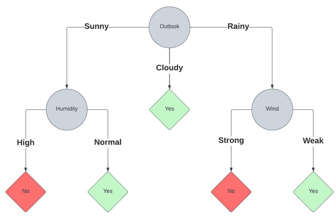
This means the node for sunny outlook will now be split in terms of humidity, and the node for rainy outlook will be split
on wind. For cloudy, the data is homogenous, it always leads to gameplay.
The process is repeated until we reach a leaf node (no more splitting), thus creating a tree:
This process can be repeated as many times as needed, and can handle multiple types of data. Depending on what kind of data, it might require preparation before you’re able to actually run through this process.
CART Decision Tree in Ruby
Now that we have a good understanding of the basics of the algorithm, let’s take a look at a very simple implementation
of a decision tree following the principles of the CART algorithm. Let’s create a DecisionTree class with a train and a predict
method that allows us to train a tree on labelled data and then make predictions on unseen data.
Our goal is to recursively split the dataset for as long as Gini Impurity can be reduced. As we have seen previously, to calculate Gini Impurity for a particular feature, we calculate the impurity for each value (index) the feature can have against the occurrence of each label:
def calculate_gini(indices, labels)
  return 0.0 if indices.empty?
  s_labels = indices.map { |i| labels[i] }
  # Gini(D) = 1 - Σ (p_i)^2
  1.0 - s_labels.group_by(&:itself).values.sum { |v| (v.length.to_f / s_labels.length)**2 }
end
We then calculate the weighted Gini Index for the feature itself in order to determine where to split:
def calc_weighted_gini(l_indices, r_indices, labels, num_samples)
  l_weight =  l_indices.length.to_f / num_samples
  r_weight =  r_indices.length.to_f / num_samples
  gini_left = calculate_gini(l_indices, labels)
  gini_right = calculate_gini(r_indices, labels)
  l_weight * gini_left + r_weight * gini_right
end
To start building the tree, we’ll set up initial values for the decision tree node:
def initialize
  @left = nil  # left child node
  @right = nil  # right child node
  @split_feature = nil  # feature to split on
  @split_threshold = nil  # threshold for the split
  @label = nil  # label for the leaf nodes
end
We can then define a train method to train the decision tree on a set of labelled data. This is a recursive algorithm,
so it’s important to consider what the stopping conditions are:
- Homogeneous data: if all data points have the same label, then we have reached a leaf node and can stop.
- There’s no data to split: if we reach a point where the subset of data can’t be split anymore, we can stop.
- Maximum depth reached: this is a custom parameter we’ll introduce. It allows us to define a maximum depth for the tree, at which point it will stop regardless of the other two conditions being met.
Let’s start defining our train method:
def train(data, labels, max_depth)
  if labels.uniq.length == 1
    @label = labels[0]
    return
  end

  if max_depth == 0 || data.empty?
    @label = labels.max_by { |label| labels.count(label) }
    return
  end
  # Tree implementation will go here
end
Now let’s start actually interacting with the data. The first thing we need to do is identify the best split. To do that, we’ll iterate over each feature and its unique values and attempt to split for each feature and threshold. We then calculate the Gini impurity index for the split and, based on it, select the best split (the one with the lowest weighted Gini index):
num_samples = data.length
num_features = data[0].length
best_gini = 1.0
best_split_feature = nil
best_split_threshold = nil
l_data = nil
l_labels = nil
r_data = nil
r_labels = nil

(0...num_features).each do |f_index|
  feature_values = data.map { |x| x[f_index] }
  feature_values.uniq.each do |threshold|
    l_indices = data.each_index.select do |i|
      data[i][f_index] <= threshold
    end
    r_indices = data.each_index.select do |i|
      data[i][f_index] > threshold
    end
    weighted_gini = calc_weighted_gini(l_indices, r_indices, labels, num_samples)

    if weighted_gini < best_gini
      best_gini = weighted_gini
      best_split_feature = f_index
      best_split_threshold = threshold
      l_data = []
      l_labels = []
      r_data = []
      r_labels = []
      l_indices.each do |i|
        l_data << data[i]
        l_labels << labels[i]
      end
      r_indices.each do |i|
        r_data << data[i]
        r_labels << labels[i]
      end
    end
  end
end
If a good split is found (best_gini < 1.0), the internal node is set to be a decision node and child nodes are created
based on the chosen split for feature and threshold. We then create new DecisionTree instances for the left and right nodes and
recursively call our train method on them. If no good split is found, the node is set to be a leaf node with the most frequent label:
if best_gini < 1.0
  # If a split reduces the Gini impurity,
  # create left and right child nodes and continue training.
  @split_feature = best_split_feature
  @split_threshold = best_split_threshold
  @left = DecisionTree.new
  @right = DecisionTree.new
  @left.train(l_data, l_labels, max_depth - 1)
  @right.train(r_data, r_labels, max_depth - 1)
else
  # If the best split doesn't reduce Gini impurity,
  # assign the most frequent label to the node.
  @label = labels.max_by { |label| labels.count(label) }
end
This concludes our train method!
For the prediction, want to give the predict method a sample to predict on and a default label in case it can’t classify
the sample (this is a very simple implementation of CART, so we’ll feed a default_label ourselves, more robust implementations can handle this).
It will first check to see if the current node is a leaf node and, if so, return the associated label. If it isn’t, it will then check if the tree might not have a left or right child for a specific sample and, in such cases, return the default label.
If, however, the current node is a decision node with a valid split threshold, it will check whether to split on the right or left node and recursively call itself until a prediction is made:
def predict(sample, default_label)
  # If it's a leaf node, return the label.
  return @label if @label

  # If not a leaf node, check the splitting criteria.
  if @split_feature.nil? || @split_threshold.nil? || sample[@split_feature].nil?
    return default_label
  end

  if sample[@split_feature] <= @split_threshold
    return @left.predict(sample, default_label) if @left
  else
    return @right.predict(sample, default_label) if @right
  end
end
Putting it all together, we have a simple CART decision tree:
class DecisionTree
  attr_accessor :left, :right, :split_feature, :split_threshold, :label

  def initialize
    @left = nil  # left child node
    @right = nil  # right child node
    @split_feature = nil  # feature to split on
    @split_threshold = nil  # threshold for the split
    @label = nil  # label for the leaf nodes
  end

  def train(data, labels, max_depth)
    if labels.uniq.length == 1
      @label = labels[0]
      return
    end

    if max_depth == 0 || data.empty?
      @label = labels.max_by { |label| labels.count(label) }
      return
    end

    num_samples = data.length
    num_features = data[0].length
    best_gini = 1.0
    best_split_feature = nil
    best_split_threshold = nil
    l_data = nil
    l_labels = nil
    r_data = nil
    r_labels = nil

    (0...num_features).each do |f_index|
      feature_values = data.map { |x| x[f_index] }
      feature_values.uniq.each do |threshold|
        l_indices = data.each_index.select do |i|
          data[i][f_index] <= threshold
        end
        r_indices = data.each_index.select do |i|
          data[i][f_index] > threshold
        end
        weighted_gini = calc_weighted_gini(l_indices, r_indices, labels, num_samples)

        if weighted_gini < best_gini
          best_gini = weighted_gini
          best_split_feature = f_index
          best_split_threshold = threshold
          l_data = []
          l_labels = []
          r_data = []
          r_labels = []
          l_indices.each do |i|
            l_data << data[i]
            l_labels << labels[i]
          end
          r_indices.each do |i|
            r_data << data[i]
            r_labels << labels[i]
          end
        end
      end
    end

    if best_gini < 1.0
      # If a split reduces the Gini impurity,
      # create left and right child nodes and continue training.
      @split_feature = best_split_feature
      @split_threshold = best_split_threshold
      @left = DecisionTree.new
      @right = DecisionTree.new
      @left.train(l_data, l_labels, max_depth - 1)
      @right.train(r_data, r_labels, max_depth - 1)
    else
      # If the best split doesn't reduce Gini impurity,
      # assign the most frequent label to the node.
      @label = labels.max_by { |label| labels.count(label) }
    end
  end

  def predict(sample, default_label)
    # If it's a leaf node, return the label.
    return @label if @label

    # If not a leaf node, check the splitting criteria.
    if @split_feature.nil? || @split_threshold.nil? || sample[@split_feature].nil?
      return default_label
    end

    if sample[@split_feature] <= @split_threshold
      return @left.predict(sample, default_label) if @left
    else
      return @right.predict(sample, default_label) if @right
    end
  end

  private

  def calculate_gini(indices, labels)
    return 0.0 if indices.empty?
    s_labels = indices.map { |i| labels[i] }
    # Gini(D) = 1 - Σ (p_i)^2
    1.0 - s_labels.group_by(&:itself).values.sum { |v| (v.length.to_f / s_labels.length)**2 }
  end

  def calc_weighted_gini(l_indices, r_indices, labels, num_samples)
    l_weight =  l_indices.length.to_f / num_samples
    r_weight =  r_indices.length.to_f / num_samples
    gini_left = calculate_gini(l_indices, labels)
    gini_right = calculate_gini(r_indices, labels)
    l_weight * gini_left + r_weight * gini_right
  end
end
Conclusion
Now we have our very own decision tree, the basis for our ensemble classification models. In the next article, we will cover the most popular ones: Random Forest Classification and Gradient Boosting Classification.
Excited about leveraging machine learning and AI in your Ruby on Rails app? We’re passionate about building interesting, valuable products for companies just like yours! Send us a message over at OmbuLabs! !